A fundamental component of the business world today is Microsoft Excel. The application records data and creates meaningful charts for visual data analysis. Nonetheless, most people have questions in Excel about how to change legend text, and also, many have found issues when taking part in some of the actions on how to change legend text in Excel. You can follow the steps if you wish to change the legend names.
- In Excel, select the Chart and click Design > select data.
- Click on the legend name & choose the data source dialog box, and click Edit.
- In the text box, enter a legend name in the series name and hit OK.
In a chart, legend names are automatically created and known by the information in the cells above each column or an entire row of data utilized for the Chart. In this article, we will dive deep into how to change legend text in Excel. Read on to know more.

Here are a few steps to follow in Excel to change the legend text.
How To Show Excel Legends On Chart
The intent of the Legend in Excel charts is to explain what type of data is visually in any colour. It is a simple square that contains a description of the paint and a description of the text.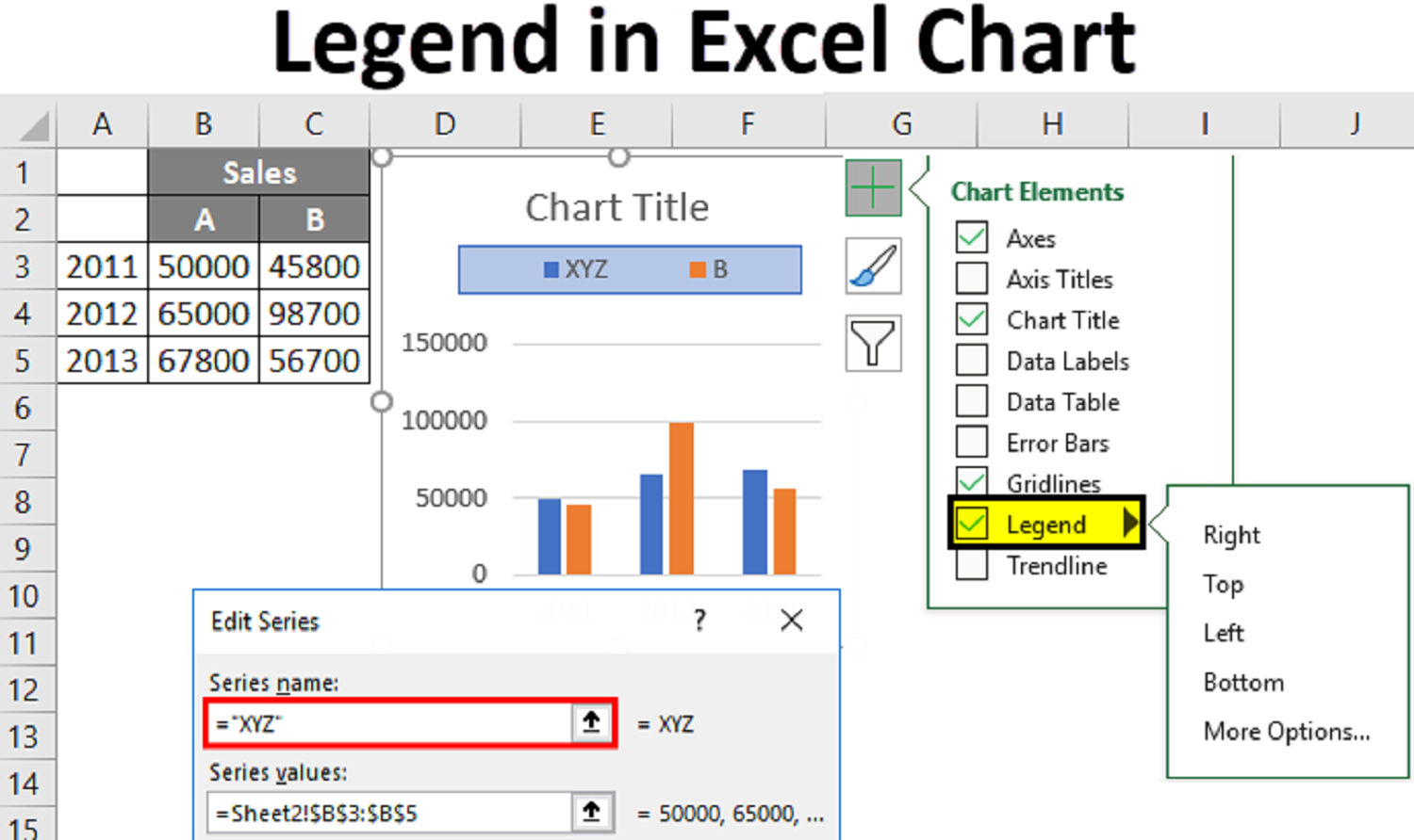
The Legend will not display when creating a chart with that data. To fix this, select the entire Chart. Then, click the plus sign button on the Chart’s right-hand side. With this on Excel, how to change the legend text can be done.
Next, you will toggle on legends from the element menu. If you want to see where the Legend is located on the Chart, click on the small black arrow on the Chart.
How to Edit Legend Entries in Excel
The Legend on a graph visually represents each data series, making it easier to understand them. The Legend changes according to the Chart’s data. Legends show what each visual label represents if the data includes many color visuals.
We can easily understand charts by using legends. Legends are automatically modified whenever we create a graph or plot our data. If we encounter an Excel chart without a legend, we can easily add one by following these steps:
- Firstly, Click anywhere on the Chart
- Click the Layout tab, then Legend
- From the Legend drop-down menu, select the position we prefer for the Legend
Then the Legend will appear on the right side.
See Also: Excel Filter Not Showing All Values? Ultimate Troubleshooting Tips
The Legend in The Chart Can Be Edited By Changing The Name or Changing its Position And Format.
Follow the below steps:
- First, Open the Excel sheet on your computer you want to edit.
- Secondly, Click on the Chart you want to edit or modify in your Excel sheet. Clicking it at the top of the spreadsheet will display the Display, layout, and format.
- Click on the Design Tab on the top of your Excel sheet, and it will display your design tools in the toolbar. (This tab name will differ based on your Excel version, some may be a Chart design).
- Click Select data in the design toolbar. This will open a new tab in which you can edit your Legend and data values.
- Select the legend entry in the “legend entries box” This box has all the legend entries on your Chart. Find the entry you edit here, click on it, and select it.
- Click on the edit button. This will help you to edit the selected entries and data names. ( In some versions of excels, you won’t be able to see the Edit button, you can instead look for the name or series name).
- You can type a new entry name in the Series name box. Double-click the text field, delete the existing name, and enter the name you want to be in that particular box.
- Enter a new chart value in the Y value box. You can delete the current data value in the box and enter a new deal in your Chart. If you have many values, use a comma to separate that.
- Click the Ok button to save your name, value edits, and apply the changes.
By this, excel how to change legend text, and the query is known. And also, you can change legend names in Excel.
Things to Remember When We Add Legend
Below are little something to remember: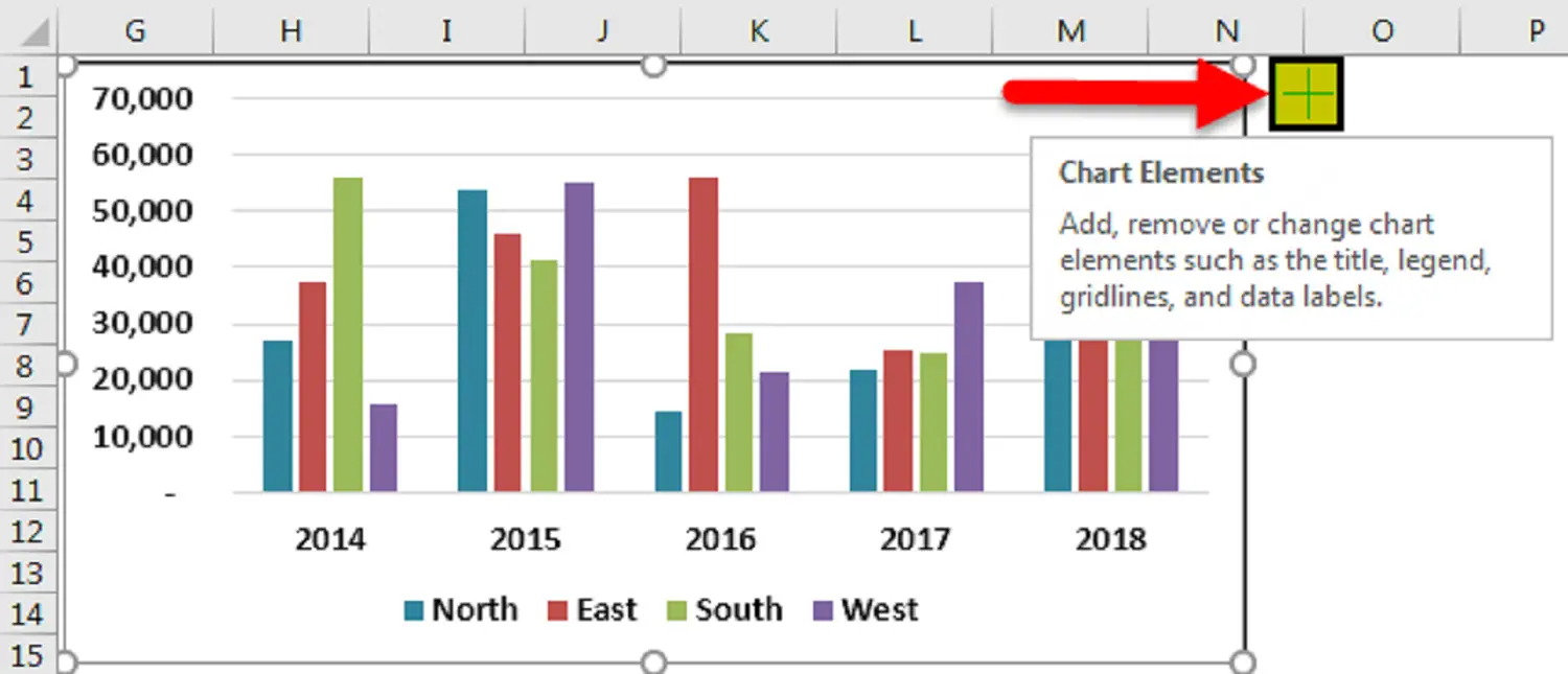
- By default, we see legends at the bottom.
- Legends are dynamic and change as per the color, texture, and text change.
- We can navigate the positioning of the Legend as per our wish but cannot place it outside the chart area.
How To Format An Excel Legend
Several options are available to modify a legend after the Display is in an Excel Chart. These options include changing the size and color and adding text effects—all the process is by right-clicking on the Legend and selecting Font from the menu. Firstly, Click on the right of the task pane to open the Format legend task panel. It has three sections with formatting options. Secondly, Now you can underline or even strikethrough your text.
Fill & Line is the first section, Effects is the second, and Legend options are the last. You can add a border to the legend text in the first section. One of the biggest challenges in making the Legend visible is to let it stand out visually using effects such as glows and shadows and controlling its location within the Chart.
This also helps in how to edit the Legend in Excel.
Use The Select Data Source Dialog
Firstly, you can select the Chart, choose the data from the menu, and use the right mouse button to access the select data source dialog box, allowing you to edit the series name. I’m sure you’ve already noticed that the Legend will change when you change the series name in Excel. In the Tools Design tab, you will find select data after you choose the Chart.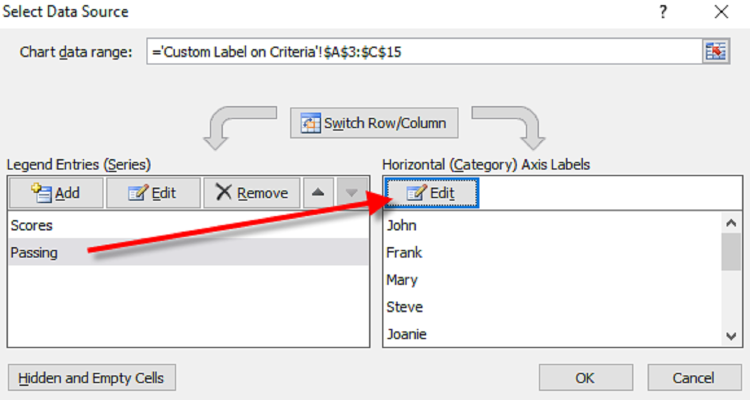
Select the Legend whose name you want to change from the Legend Entries or the series list. Secondly, click Edit Button and type a name into the series name text box. Finally, click OK to dismiss the box with your new legend name.
Once you have done that, select the Data Source dialogue, and the legend name is updated. And also, Please note that changing the legend name will not change the text containing the data in the column.
Using this one of the methods, excel, how to change legend text can be solved.
Find out: How To Repair Corrupted Excel File In 2024?
FAQ’s
Can you edit the text of the Legend in Excel?
Yes, using the Design tab in the data section, click select data. In the data source dialog box, in the legend entries, choose the legend entry you want to change.
How to remove or how to change legend labels in excel?
Right-click on the series you want to hide and select hide properties. Select Legend and select the do not show legend option.
Conclusion
In conclusion, Here is the guide on changing legend text, formatting an Excel legend, using the select data source dialog, and showing legend text. There are numerous steps to follow, changing the legend name in Excel, etc. Ensure that you follow every step carefully.

Mauro Huculak: Technical writer specializing in Windows 10 and related technologies. Microsoft MVP with extensive IT background and certifications.